Spark Shuffle Explained: Why Wide Transformations Slow Your Job
A shuffle moves data across the network between executors. It is also the root cause of the three problems people spend most of their time debugging: skew, spill and out of memory errors.
Most Spark performance problems trace back to one operation: the shuffle.
Skew, spill and out of memory errors are not three separate topics. They are three ways the same operation goes wrong. Understand the shuffle and all three stop being mysterious.
First: how Spark stores your data
To understand a shuffle, you need one thing clear first — and it is the thing most explanations skip.
Your table is not sitting in one place.
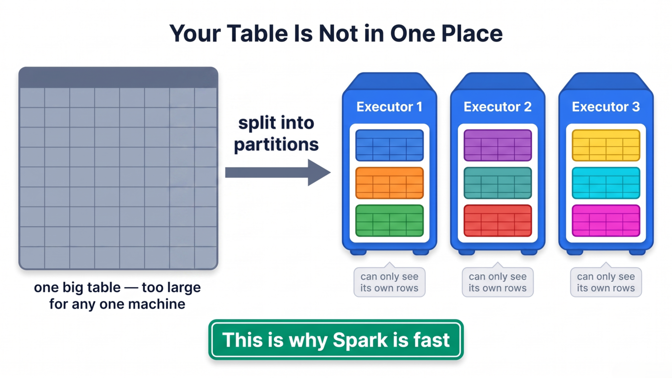
When Spark reads a large table, it does not load it into one machine. It cannot — the table is bigger than any single machine. So Spark cuts it into pieces called partitions, and hands those pieces out to different machines called executors.
A partition is a chunk of your rows.
An executor is one machine in the cluster.
Each executor holds some partitions and works only on those.
This is the entire reason Spark is fast. Ten machines each working on a tenth of your data finish roughly ten times sooner than one machine working on all of it.
But it comes with a catch, and the catch is the whole story: an executor can only see the rows it is holding. It has no idea what is on the other machines.
Your table is cut into partitions and spread across machines. Each machine only sees its own rows.
Why that becomes a problem
Say you have 12 sales rows spread across three executors, and you want a count per country.
df.groupBy("country").count()
Here is where the rows happen to be sitting:
Executor
Rows it is holding
Executor 1
US, India, US, UK
Executor 2
India, UK, US, India
Executor 3
UK, US, India, UK
Now ask Executor 1: how many US rows are there?
It looks at what it holds and says 2.
That answer is wrong. The real total is 4 — there is one more US row on Executor 2 and another on Executor 3. Executor 1 cannot see them, so it cannot possibly give the right answer.
And this is not a bug you can code around. No executor can answer the question, because no executor has all the rows for any single country.
There is only one way out. The rows have to be moved so that all the rows sharing a country end up on the same machine.
Executor
Before
After the move
Executor 1
US, India, US, UK
US, US, US, US
Executor 2
India, UK, US, India
India, India, India, India
Executor 3
UK, US, India, UK
UK, UK, UK, UK
Now every executor can answer correctly on its own: US = 4, India = 4, UK = 4. Same 12 rows, sitting in different places.
That move is the shuffle.
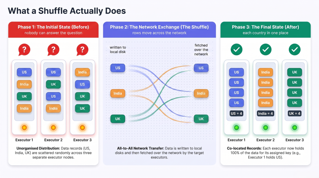
Before: every country is on every machine, so nobody can count. After: each country is in one place.
So when you read the textbook definition — “a shuffle redistributes data across partitions, exchanging it over the network between executors” — that is all it means. Rows get re-sorted onto machines according to their key, so that matching rows end up together.
One honest note on the example: for a simple count, Spark is smart enough to add up each executor’s partial totals first and move only those small numbers. But the principle is identical, and for most operations — joins, sorting, distinct — the actual rows really do have to travel.
And travelling is expensive. Moving rows means writing them to disk, sending them over the network to another machine, and reading them back. That is why the shuffle is the most expensive thing Spark does.
Narrow vs wide transformations
Now the useful question: which operations force this move, and which do not?
Every Spark transformation is one of two kinds.
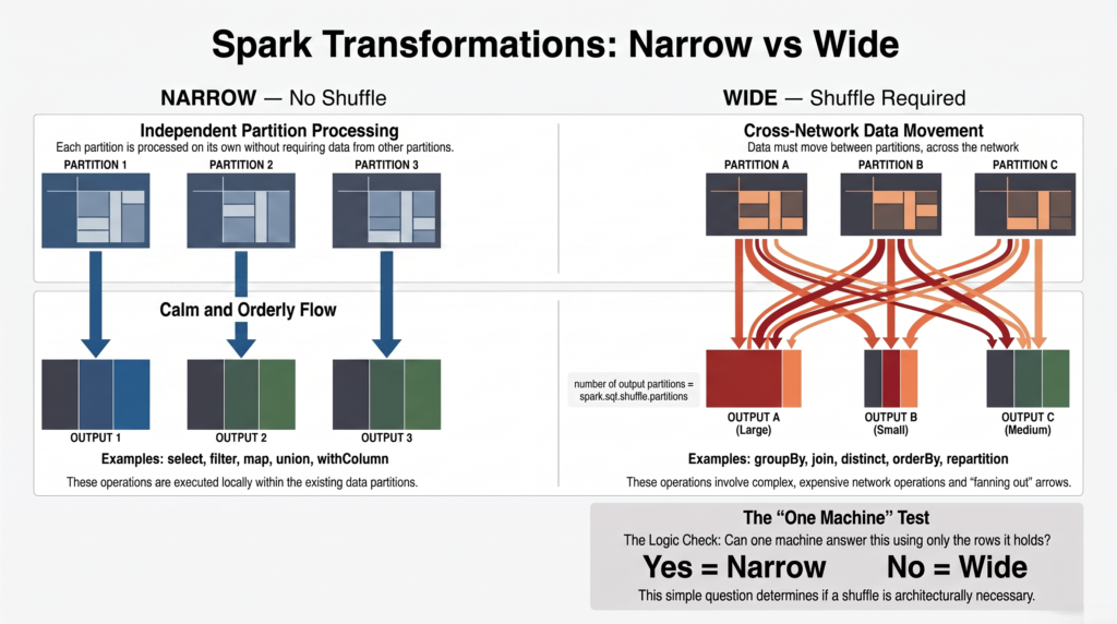
Narrow transformation — operates on data within a single partition, without requiring any data to move. Each executor can finish its own rows without asking anyone else anything.
Wide transformation — requires data to be shuffled between partitions. The output is repartitioned, and the number of output partitions is controlled by spark.sql.shuffle.partitions.
Narrow
Wide
Data movement
None
Across the network
Works on
One partition at a time
Data from all partitions
Cost
Cheap
Expensive
Creates a new stage
No
Yes
Examples
select, filter, map, union, withColumn
groupBy, join, distinct, orderBy, repartition
The test is simple. Ask: can one executor answer this by looking only at its own rows?
“Keep rows where country = US” — yes. Each executor checks its own rows. Narrow.
“Count rows per country” — no. It needs rows from everywhere. Wide.
# Narrow - no shuffle. Every partition handled independently.df.filter(df.country =="US")df.select("id", "amount")df.withColumn("total", df.price * df.qty)# Wide - shuffle required. Data must move.df.groupBy("country").count()df.join(other_df, "customer_id")df.distinct()df.orderBy("amount")
Narrow: each partition processed on its own. Wide: data moves between partitions across the network.
What actually happens during a shuffle
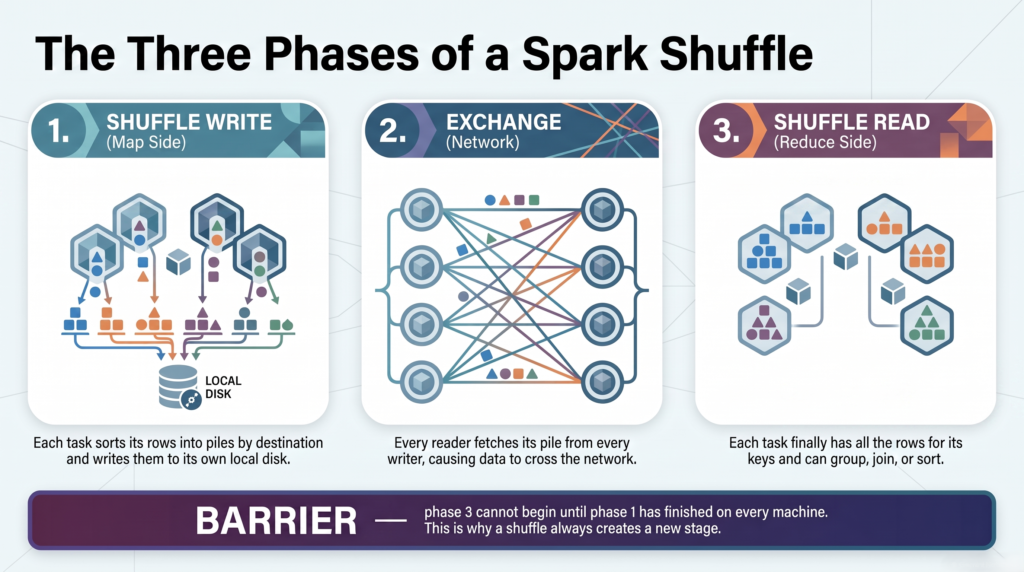
The move happens in three phases.
Shuffle write (map side). Each task takes its partition and sorts the rows into piles by where they need to go — usually by hashing the join or group key. It writes those piles to local disk on its own executor.
Exchange (network transfer). The tasks in the next stage each fetch their own pile from every executor that wrote one. This is where data crosses the network.
Shuffle read (reduce side). Each task now holds all the rows for its keys, and can finally do the grouping, joining or sorting.
Two things follow from this that explain a lot of Spark behaviour.
A shuffle is a barrier. Phase 3 cannot start until phase 1 has completely finished everywhere, because a task cannot know it has all its rows until every writer is done. This is why Spark splits a job into stages at every shuffle — the boundary between two stages is always a shuffle. See Spark Architecture Explained Simply for how jobs, stages and tasks fit together.
Shuffle write is not the same as spill. Writing shuffle files to local disk is normal and always happens. Spill is something else, and we come to it below.
Write to local disk, fetch across the network, then read. Nothing downstream can start until the write finishes.
How many partitions come out?
The number of output partitions after a shuffle is set by spark.sql.shuffle.partitions, which defaults to 200.
That number is fixed regardless of your data volume, which causes trouble at both extremes:
Small dataset, 200 partitions — tiny tasks, scheduling overhead, and 200 tiny output files if you write straight after. That is one of the main sources of the small files problem.
Huge dataset, 200 partitions — each partition is enormous, which leads directly to spill and out of memory errors.
On Spark 3.x, Adaptive Query Execution largely solves this by adjusting the partition count at runtime based on the actual data. If AQE is enabled, you generally should not tune this setting by hand.
The three problems a shuffle causes
This is why the shuffle matters so much. Almost every Spark performance issue is one of these three, and all three start here.
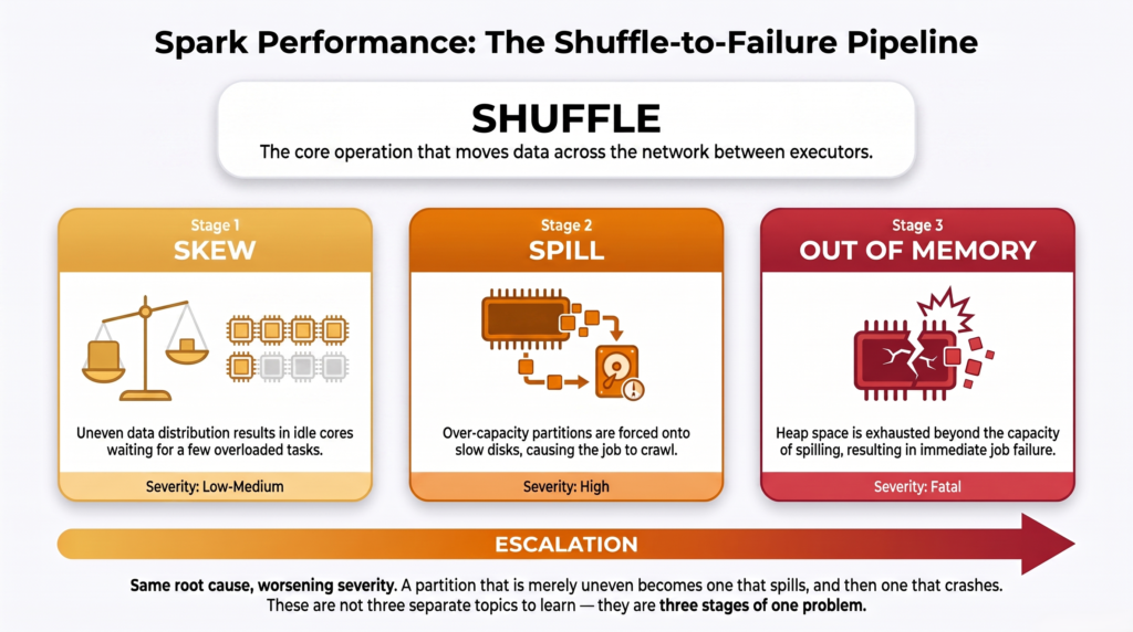
Skew, spill and OOM are not three separate topics. They are three ways a shuffle goes wrong.
1. Skew
Data skew occurs when some partitions receive significantly more data than others.
This imbalance causes certain tasks to take much longer to complete, slowing down the whole job.
Go back to the country example. That worked neatly because each country had four rows. Real data is never that tidy. If 40% of your rows are US, then after the shuffle one machine is holding 40% of the entire dataset while others hold almost nothing.
And because a stage only finishes when its slowest task finishes, 199 tasks sit idle waiting for one.
Skew also makes the other two problems worse — that oversized partition is the one most likely to spill or run out of memory.
During a shuffle, if the data being processed exceeds the executor’s memory, it spills to disk.
Disk is much slower than memory, so performance degrades badly.
Here is the distinction that trips people up. Shuffle write is Spark deliberately writing shuffle files to local disk — normal, happens every time. Spill is Spark running out of room while processing and dumping its working data to disk as an emergency measure. One is by design. The other is a symptom.
Spill is the quiet killer. Your job does not fail — it just gets slower, sometimes by an order of magnitude, with no error to point at.
You can see it directly in the Spark UI: the Spill (Memory) and Spill (Disk) columns in a stage’s Summary Metrics. On a healthy stage they are zero.
3. Out of memory
If the data is too large for the executor’s memory and spilling is not sufficient, the job fails with an Out of Memory error.
This happens when shuffle data or intermediate results are simply too large to fit.
Think of the three as an escalation. A partition is too big → tasks are uneven (skew). Too big for memory → it spills (slow). Too big even to spill safely → it crashes (OOM).
One thing worth being clear about: this is executor OOM, caused by shuffle data. It is a different problem from driver OOM, which is usually caused by pulling data back with collect() or broadcasting something too large— covered in Spark Driver OOM.
Seeing shuffles in the Spark UI
Open the Spark UI and go to the Stages tab.
Look at the Shuffle Read and Shuffle Write columns. Any stage with numbers there performed a shuffle.
Click into the slowest stage and open Summary Metrics.
Summary Metrics is the most useful table in the Spark UI, because it shows each metric at the Min, 25th percentile, Median, 75th percentile and Max. Comparing those columns tells you which of the three problems you have.
Summary Metrics for a skewed stage: median shuffle read of 0 B, max of 1.7 GiB, and spill appearing only in the top quartile.
In that example the Shuffle Read Size row reads 0 B at the median and 1.7 GiB at the maximum. Most tasks received nothing; one received 1.7 GiB. Task duration tells the same story — 11 ms at the median, 1.2 minutes at the max. And the spill columns are zero until the 75th percentile, then jump to 3.8 GiB. That is skew causing spill, exactly as described above.
What Summary Metrics shows
What it means
Max shuffle read much larger than Median
Skew
Spill (Memory) or Spill (Disk) not zero
Spill — partitions too large for memory
Percentiles all similar, all slow
Not a shuffle problem. Look inside the task.
Everything even and fast
The shuffle is healthy
That third row matters. If every task is equally slow, the shuffle is fine and something inside the task is expensive — a Python UDF, for example, which serializes data out of the JVM on every row. That is covered in PySpark Data Serialization.
How to reduce shuffling
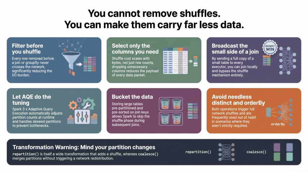
You cannot remove shuffles entirely — joins and aggregations need them. But you can make them smaller, rarer, or avoid them in specific cases.
Filter before you shuffle. The cheapest fix on the list. Every row you remove before a join or groupBy is a row that never crosses the network. Spark’s optimiser pushes filters down automatically where it can, but it cannot push one through a UDF.
Select only the columns you need. Shuffle cost scales with bytes, not rows. Dropping unused columns before a wide transformation shrinks every phase of the shuffle.
Broadcast the small side of a join. If one table is small enough to fit in each executor’s memory, Spark can send a full copy to every executor and join locally — no shuffle at all. This is the single biggest win available on join-heavy jobs.
Let AQE do the tuning. On Spark 3.x, Adaptive Query Execution adjusts partition counts at runtime, converts joins to broadcast joins when it discovers a side is small, and splits skewed partitions automatically.
Pre-shuffle the data with bucketing. If two large tables are joined on the same key repeatedly, bucketing stores them already partitioned and sorted on that key, so the join can skip the shuffle.
Avoid unnecessary wide operations.distinct() and orderBy() both trigger full shuffles and are often used out of habit. Sorting a dataset you are only going to aggregate afterwards is wasted work.
One more that is easy to get wrong: repartition() is itself a wide transformation and triggers a full shuffle, while coalesce() merges partitions without one. Reaching for repartition to “fix” performance often adds a shuffle rather than removing one — see repartition vs coalesce.
You cannot remove every shuffle. You can make them carry far less data.
Quick reference
Question
Answer
Why is data split up at all?
So many machines can work on it at once. That is what makes Spark fast.
What is a shuffle?
Moving rows between machines so that matching rows end up together
Why is it needed?
An executor can only see its own rows, so it cannot answer questions about the whole table
What triggers one?
Any wide transformation — groupBy, join, distinct, orderBy, repartition
Spark splits your table into partitions and spreads them across executors. Each executor only sees its own rows.
Some questions cannot be answered from one machine’s rows alone — like counting per country when every country is on every machine.
So Spark moves the rows around until matching ones are together. That move is the shuffle.
Wide transformations cause shuffles. Narrow transformations do not.
It runs in three phases: write to local disk, fetch across the network, then read. Nothing downstream starts until the write finishes, which is why a shuffle always creates a new stage.
Three problems come out of it: skew when partitions are uneven, spill when a partition is too big for memory, and OOM when spilling is not enough to save it.
You cannot eliminate shuffles, but filtering early, selecting fewer columns, broadcasting small tables and enabling AQE all make them cheaper.
Frequently Asked Questions
What is a shuffle in Spark?
A shuffle is Spark moving rows between machines so that related rows end up together. It is needed because your table is split into partitions spread across executors, and each executor can only see its own rows. Operations like groupBy and join need rows that may be on other machines, so the data has to be redistributed over the network first.
Why does Spark split data into partitions?
Because a large table will not fit on one machine, and because splitting it lets many machines work in parallel — ten machines each handling a tenth of the data finish roughly ten times sooner. The trade-off is that no single machine has the full picture, which is exactly why shuffles become necessary.
What is the difference between narrow and wide transformations?
A narrow transformation operates on data within a single partition and needs no data movement — select, filter, map, union and withColumn are narrow. A wide transformation requires shuffling data between partitions and produces output partitioned according to spark.sql.shuffle.partitions — groupBy, join, distinct and orderBy are wide. The test: can one executor answer using only its own rows?
Why is shuffle expensive in Spark?
Because it combines the three slowest things a distributed system does: writing to disk, serializing data, and sending it over the network. It is also a barrier — no task in the next stage can begin until every task in the previous one has finished writing, so the whole cluster waits for the slowest writer.
What problems does shuffling cause?
Three. Skew, where some partitions receive far more data than others so a few tasks run much longer. Spill, where a partition exceeds the executor’s memory and gets written to disk, which is far slower. And out of memory errors, where the data is too large even for spilling to rescue and the job fails.
Is shuffle write the same as spill?
No, and confusing them causes wasted debugging. Shuffle write is Spark deliberately writing shuffle files to local disk, which happens on every shuffle by design. Spill is Spark running out of memory while processing and dumping working data to disk as an emergency measure. Shuffle write is normal; spill is a symptom.
What is spark.sql.shuffle.partitions?
It sets how many partitions are produced after a shuffle, defaulting to 200. Because it is fixed regardless of data volume, it creates tiny wasteful partitions on small datasets and enormous ones on large datasets. On Spark 3.x, Adaptive Query Execution adjusts this at runtime, so manual tuning is usually unnecessary.
How do I see shuffles in the Spark UI?
Go to the Stages tab and look at the Shuffle Read and Shuffle Write columns — any stage with values there performed a shuffle. Then click into the slowest stage and open Summary Metrics, which shows each metric at Min, 25th, Median, 75th and Max. Comparing Median against Max is how you tell skew from spill.
How can I avoid a shuffle in a join?
If one table is small enough to fit in executor memory, broadcast it — Spark sends a full copy to every executor and joins locally with no shuffle. For two large tables joined repeatedly on the same key, bucketing stores them pre-partitioned and pre-sorted so the shuffle can be skipped. Otherwise reduce the shuffle rather than remove it, by filtering and selecting fewer columns first.
Does repartition cause a shuffle?
Yes. repartition() is a wide transformation and performs a full shuffle to redistribute data evenly. coalesce() merges existing partitions without a shuffle, which makes it cheaper but can leave uneven partition sizes. Using repartition to fix a slow job often adds a shuffle instead of removing one.